
If your supervisor told you to multiply your biggest construct by ten, that rule has been tested and it fails badly — in one published comparison it recommended 20 respondents where the true minimum was 599. Here is the method reviewers now expect, the exact G*Power steps, and a lookup table so you can find your number without opening the software.
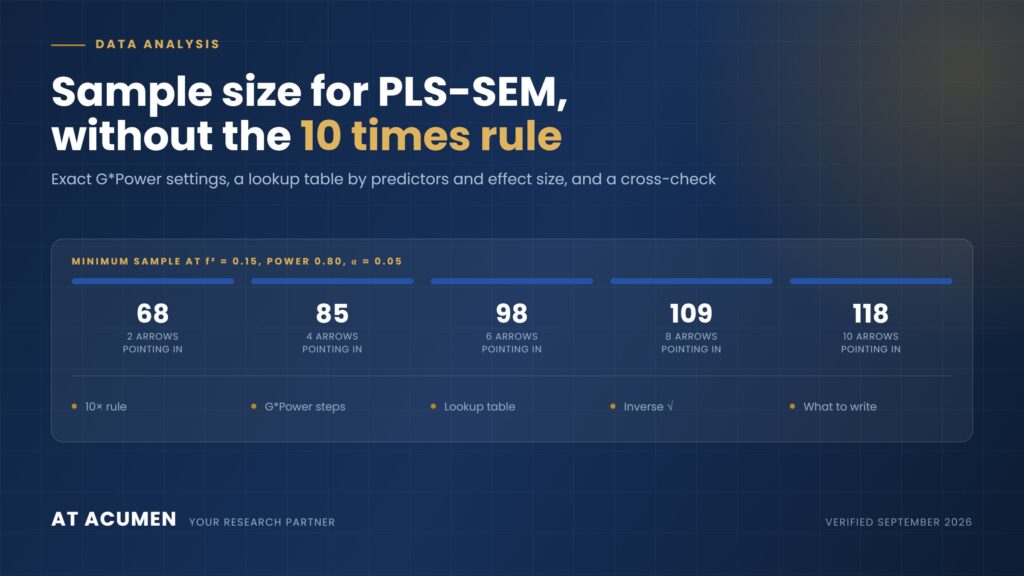
The short version. Count the arrows pointing into your most-predicted construct. That count is your number of predictors. Run an a priori power analysis for linear multiple regression at α = 0.05, power = 0.80 and f² = 0.15. For five predictors that returns 92.
Why the “10 times rule” has to go
The rule comes from Barclay, Higgins and Thompson (1995): sample size should be at least ten times the larger of the most formative indicators on a construct, or the most structural paths aimed at a construct. It became folklore because PLS-SEM is tolerant of small samples, and people read tolerance as permission.
Kock and Hadaya (2018) tested it directly in three Monte Carlo experiments. The rule produced the same answer every time — N = 20 — while the true minimums were:
| Scenario | 10 times rule says | True minimum | Achieved power |
|---|---|---|---|
| 1 | 20 | 28 | ≈ 0.65 |
| 2 | 20 | 265 | far below 0.30 |
| 3 | 20 | 599 | far below 0.30 |
Even in the mildest scenario the rule delivers power of about 0.65 against a conventional target of 0.80. Goodhue, Lewis and Thompson made the same point in MIS Quarterly in 2012, and Marcoulides and Saunders had warned about it in 2006. If a reviewer knows the field, “we followed the 10 times rule” invites a question you do not want.
What to do instead
Hair et al. are explicit in the PLS-SEM primer: sample size “should be determined by means of power analyses based on the part of the model with the largest number of predictors.”
In practice that means one thing — look at your model and find the construct with the most arrows pointing at it. Count them. Include both structural paths and formative indicators. That number, and nothing about your total sample or your number of constructs, is what drives the calculation.
The exact G*Power steps
- Test family:
F tests - Statistical test:
Linear multiple regression: Fixed model, R² deviation from zero - Type of power analysis:
A priori: Compute required sample size — given α, power, and effect size - Effect size f²:
0.15for a medium effect. Cohen’s conventions are 0.02 small, 0.15 medium, 0.35 large. - α err prob:
0.05 - Power (1−β err prob):
0.80 - Number of predictors: your arrow count from the step above
- Click Calculate. Read Total sample size.
The lookup table
Minimum sample size at α = 0.05, by number of predictors and effect size.
| Predictors (arrows in) |
f² = 0.02 small |
f² = 0.15 medium |
f² = 0.35 large |
f² = 0.15 at power 0.90 |
|---|---|---|---|---|
| 2 | 485 | 68 | 31 | 88 |
| 3 | 550 | 77 | 36 | 99 |
| 4 | 602 | 85 | 40 | 108 |
| 5 | 647 | 92 | 43 | 116 |
| 6 | 688 | 98 | 46 | 123 |
| 7 | 725 | 103 | 49 | 130 |
| 8 | 759 | 109 | 52 | 136 |
| 9 | 791 | 114 | 54 | 141 |
| 10 | 822 | 118 | 57 | 147 |
Scroll the table sideways on mobile. Power is 0.80 except in the final column.
How we produced this table, so you can check it. We computed each value from the noncentral F distribution using the same algorithm G*Power implements — critical F at the given α, non-centrality parameter λ = f² × N, and degrees of freedom of k and N − k − 1. We validated the method against the worked example published in the G*Power reference paper itself: Faul et al. (2009) report that 3 predictors, f² = 1, α = 0.05 and power = 0.95 requires N = 22. Our calculation returns 22 exactly, and 21 falls short. Open G*Power and confirm your own row before you cite it.
Read the small-effect column before you decide
Most students set f² = 0.15 because a tutorial told them to, and never look at the first column. That column is the honest one. If you genuinely expect small effects — common in behavioural research with many controls — five predictors demands 647 responses, not 92.
Choosing f² is a substantive decision, not a default. Base it on effect sizes reported in comparable published studies in your field, and say in your methods chapter which studies you based it on. That single sentence is what separates a justified sample size from a number someone picked.
The second method: inverse square root
Kock and Hadaya (2018) proposed a simpler alternative that needs no software:
N > (2.486 / |β|min)²
Where |β|min is the absolute value of the smallest path coefficient you expect to be statistically significant. The constant 2.486 is z.95 + z.80 — that is, 1.645 + 0.842 — which fixes power at 0.80 and α at 0.05.
| Smallest expected path |β| | 0.10 | 0.15 | 0.20 | 0.25 | 0.30 | 0.40 |
|---|---|---|---|---|---|---|
| Minimum N | 619 | 275 | 155 | 99 | 69 | 39 |
Note how sensitive this is. Expecting to detect a path of 0.10 rather than 0.20 quadruples your sample. If your model has one weak hypothesised link and you want to claim it, that link sets your sample size.
Kock and Hadaya also describe a gamma-exponential method, which corrects a known bias in the inverse square root estimate. In their own simulations the gamma-exponential figures (26, 273, 605) tracked the true minimums (28, 265, 599) closely, while the 10 times rule did not come near.
Which should you use?
They answer different questions. G*Power asks how large a sample you need to detect a given effect size in the most complex regression. The inverse square root method asks how large a sample you need to detect a given path coefficient. Neither is the other’s approximation — Kock and Hadaya’s paper does not mention G*Power at all.
The practical answer for a thesis: report both, and take the larger. It costs you two sentences and removes an obvious line of attack.
What to actually write in your thesis
Minimum sample size was determined using an a priori power analysis for the most complex regression in the structural model, which contained five predictors (Hair et al., 2022). Using G*Power 3.1 (Faul et al., 2009) with f² = 0.15, α = 0.05 and power = 0.80, the required sample size was 92. As a cross-check, the inverse square root method (Kock & Hadaya, 2018) with a minimum expected path coefficient of 0.20 indicated a minimum of 155. The larger figure was adopted, and 187 usable responses were obtained.
Replace the numbers with yours. Keep the structure — it states the method, the parameters, the source, the cross-check and the outcome, which is exactly what an examiner is checking for.
Need a sample size you can defend in a viva?
We work with postgraduate researchers on power analysis, sampling justification and PLS-SEM model assessment — on your own model, with numbers you can explain.
Related: HTMT discriminant validity: is the threshold 0.85 or 0.90?
Sources
Barclay, D. W., Higgins, C. A., & Thompson, R. (1995). The partial least squares (PLS) approach to causal modeling. Technology Studies, 2(2), 285–309.
Cohen, J. (1992). A power primer. Psychological Bulletin, 112(1), 155–159.
Faul, F., Erdfelder, E., Buchner, A., & Lang, A.-G. (2009). Statistical power analyses using G*Power 3.1: Tests for correlation and regression analyses. Behavior Research Methods, 41(4), 1149–1160.
Goodhue, D. L., Lewis, W., & Thompson, R. (2012). Does PLS have advantages for small sample size or non-normal data? MIS Quarterly, 36(3), 981–1001.
Kock, N., & Hadaya, P. (2018). Minimum sample size estimation in PLS-SEM: The inverse square root and gamma-exponential methods. Information Systems Journal, 28(1), 227–261.
Marcoulides, G. A., & Saunders, C. (2006). PLS: A silver bullet? MIS Quarterly, 30(2), iii–ix.
Hair, J. F., Hult, G. T. M., Ringle, C. M., & Sarstedt, M. A Primer on Partial Least Squares Structural Equation Modeling (PLS-SEM). Sage.
Table values computed September 2026 and validated against the published example in Faul et al. (2009). Confirm your own row in G*Power before citing it.